Dependencies and halos
A halo is the extra input read around a block’s owned output. Different halo forms exist because different algorithms depend on different regions: a Gaussian filter needs nearby pixels, a directional stencil needs more on one side, an exact distance sweep needs a complete line, and an image warp needs a region in another coordinate system. Treating all of these as one symmetric radius either reads too much or loses a dependency.
This chapter uses half-open intervals: [10,20) contains indices 10 through 19. Three-dimensional shapes and axis lists are in z,y,x order.
Requirement, allocation and ownership are different
The algorithm declares a reach: the input required to compute an output. The plan grants a halo: the extra extent actually provisioned around a core. Both can be represented by Reach, but they must be derived independently. If an operation computes its required reach from whichever halo it received, the correctness check would compare a number with itself.
For one interior axis, let the owned core be [c0,c1), the granted lower/upper halo be (g0,g1), and the algorithm’s required reach be (r0,r1). The read is [c0-g0,c1+g1), clipped to the real image domain. Away from true image edges, the trustworthy interval is the read shrunk by (r0,r1); the valid output is its intersection with the core. These calculations live in BlockGeometry::derive_with.
For core [10,20), required reach (2,2), and granted halo (1,1), the read is [9,21) but only [11,19) is trustworthy. The missing edge outputs do not silently become zero or inherit a fake boundary condition: the decomposition’s exact-tiling check rejects the missing coverage.
The core is what this task owns. Halos may overlap, but ownership must not. A wide read does not authorize writing into a neighbor’s core.
Which dependency form should an operation use?
Reach combines a coordinate space with three AxisReach values. Zero, symmetric and asymmetric finite support are all instances of the bounded form; they are not separate algorithms or separate executors.
| Requirement | Why this form exists | Shipped examples |
|---|---|---|
| Zero spatial reach | Each output reads only co-located values, or reads no image | VoxelwiseMapOp, channel arithmetic through TupleOp |
| Uniform bounded reach | A fixed local neighborhood applies at every output | SmoothOp, direct filtering through ConvolveOp |
| Asymmetric bounded reach | The input support or ownership rule is directional | Anchored kernels through Kernel, morphology through MorphologyOp, positive-face evidence through RagBlockOp |
| Per-block halo table | Sampling alignment or fixed input extents require different margins at different block positions | Resample::halo, LocalStatistic::halo |
| Tile-aligned reach | A volume-anchored computational tile can require extra context when a compute block cuts through it | TransformConvolveOp, TransformBankOp |
| Whole-axis requirement | No finite local radius can reproduce the exact algorithm | DistanceSweepOp, plane FFTs through DestripeOp and DicIntegrateOp |
| Explicit source-region mapping | Output and input coordinates differ; output-space padding cannot describe the fetch precisely | WarpOp, PlaneSampleOp, lattice and stated-extent resampling routes |
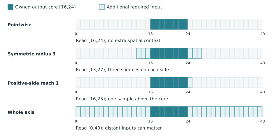
These declarations are the starting point. An execution shell may conservatively widen a fetch. For example, the fragment-phase builder currently combines source requirements into a symmetric per-axis halo; an asymmetric source declaration does not imply that every execution route already fetches its mathematically tightest one-sided region.
Bounded support: local filters and directional neighborhoods
Symmetric support
AxisReach::Bounded stores separate lower and upper distances. When they agree, it is the familiar radius. A Gaussian with sigma 1 and truncation 3 has radius ceil(3 × 1) = 3; SmoothOp needs three input voxels on either side of each output on that axis. With anisotropic sigma [2,1,1], the corresponding radii are [6,3,3]. There is no reason to inflate all three axes to six.
A pointwise map is the same representation with both distances zero. It can still have several image inputs. TupleOp reads co-located channel values; zero reach describes the spatial relationship, not the number or byte size of its operands.
The reach belongs to the implemented numerical algorithm. A Gaussian has infinite mathematical support, but the implemented truncated kernel has finite support. Conversely, choosing a small radius does not turn an exact global algorithm into a local one without changing its result.
Asymmetric support
For the backward difference y[i] = x[i] - x[i-1], the lower reach is one and the upper reach zero. Granting (1,1) remains sufficient, but fetches an unused face. Granting (0,1) is wrong: it reads the opposite neighbor. In three large dimensions, unnecessary faces multiply the read volume.
Anchored convolution makes this distinction concrete. Kernel::reach_spec uses the kernel support and Sense. Correlation with support (lo,hi) = (1,4) reads one position below and four above an output; convolution reverses the kernel and swaps those requirements. A symmetric maximum (4,4) hides the orientation and overreads. Reusing the correlation’s asymmetric declaration for convolution underreads one side.
Morphological elements can also have uneven or off-center support. MorphologyOp derives its requirement from the operation and the element, rather than assuming that its bounding box has an odd extent centered on each output. RagBlockOp uses a different reason for directionality: comparing only positive faces gives each adjacent voxel pair one owner. It declares the needed positive-side windows on its label and evidence SourceInput values.
Per-block tables: a requirement can be uniform while its grant varies
AxisReach::PerBlock stores one (lo,hi) pair per block index along an axis. It is a recorded table, not a callback depending on image intensities. The plan can serialize and hash it, and Reach::check_lattice requires the table length to equal the number of blocks on that axis. This is a separable table per axis, not an arbitrary three-dimensional source box per task; nonseparable mappings use explicit source regions instead.
One use is holding the fetched extent fixed at image edges. A symmetric padding of two around an eight-pixel core gives a twelve-pixel interior read but only ten pixels at the first and last image blocks. Reach::window can instead slide the window inward:
| Core in an image of length 32 | Granted (lo,hi) |
Read interval | Read length |
|---|---|---|---|
[0,8) |
(0,4) |
[0,12) |
12 |
[8,16) |
(2,2) |
[6,18) |
12 |
[16,24) |
(2,2) |
[14,26) |
12 |
[24,32) |
(4,0) |
[20,32) |
12 |
The required stencil is still checked separately. This helper does not make an insufficient twelve-pixel window correct for an arbitrary algorithm.
A second use is a globally anchored sampling lattice. With rational resampling, a read boundary must align to the factor’s input/output correspondence. The extra distance needed to snap the lower boundary can differ from the upper boundary and from the next block’s distances. Resample::halo computes those pairs; taking the largest individual radius and applying it everywhere does not in general preserve the required boundary alignment.
LocalStatistic::halo addresses a related problem. Interpolation between sampled local statistics needs the samples bracketing each owned output, plus the window around those sample positions. If the sampling points are unevenly spaced or do not align with compute blocks, those margins depend on block position. The local-statistics reference explains when sampling can reduce computation and when the sample image is materialised.
Aligned support: why FFT tiles need two answers
AxisReach::Aligned records a tile stride and two pairs: the requirement when the compute block edge is divisible by the stride, and the conservative requirement when it is not. TransformConvolveOp anchors its FFT computation tiles to the volume, so neighboring compute decompositions use the same computational tile origins.
If a core starts in the middle of one of those tiles, computing its first owned output can require the tile’s earlier input. The additional support is not a larger PSF: it is a consequence of where the implementation’s tiles start. TransformBankOp has the same geometry while sharing an input transform among multiple correlations.
For tile stride 32 and kernel reach (3,3), AxisReach::aligned records:
| Compute block edge | Resolved reach | Interior one-axis read length |
|---|---|---|
| 64, divisible by 32 | (3,3) |
64 + 6 = 70 |
| 63, not divisible by 32 | (34,34) |
63 + 68 = 131 |
This is geometric accounting, not a measured speed ratio. The full cost also depends on clipping, dimensions, cache reuse and FFT workspace.
Why store both pairs rather than only the stride and one radius? Composition must preserve both cases. Two such operators in a sequence need (6,6) in the aligned case and (68,68) in the unaligned case. Adding just one stride - 1 penalty to the combined kernel reach would produce (37,37) and understate the unaligned requirement. Reach::in_voxels resolves the alignment once a candidate BlockGrid is known; code without a grid uses the conservative answer.
Whole-axis dependencies
AxisReach::All means that the algorithm consumes the complete axis. It is more informative than an arbitrary integer that happens to exceed today’s image size. The planner can recognize an uncuttable dimension before trying candidate block shapes.
The exact Euclidean distance transform illustrates why. In an axis sweep, the best seed for an output can lie arbitrarily far along that line. A fixed-radius window can return the right value for a small fixture and fail when a more distant seed becomes the optimum. DistanceSweepOp therefore declares the whole swept axis and zero reach on the other two. Three sweeps use different whole axes; each can keep its transverse dimensions in smaller strips. This is different from requiring the entire 3D volume at once.
Frequency-domain plane operations have another reason. DestripeOp and DicIntegrateOp use complete y/x planes while independent z planes can be processed separately. SplineCoefficientsOp similarly requires complete lines for its tridiagonal coefficient solve, but its current fragment interface expresses that by returning the axis length from its integer reach method, rather than constructing a pixel-operation AxisReach::All value.
Global flooding is a stronger requirement: SeededWatershedOp and ScalableWatershedOp declare all three axes because their shared queue can propagate decisions across the volume. A planned whole-volume operation is not therefore a bounded-memory operation. Alternative tiled watershed algorithms change the partitioning semantics; they do not acquire the same global answer merely by selecting a modest overlap.
Coordinate space: why an output halo cannot describe every input read
Space identifies the frame, units and axis order of a requirement. It avoids confusing one voxel of a coarse image with one voxel of a fine image.
| Field | Meaning | Consequence |
|---|---|---|
Frame::Phase |
Coordinates of the phase’s own volume | A clipped boundary can be a true image boundary. |
Frame::Source |
The image being read | An output crop edge is not automatically a true source boundary. |
Units::Voxels |
Distances in the stated voxel frame | Finite margins can grow a read extent directly. |
Units::Blocks |
Neighboring blocks in a lattice | Conversion needs the chosen block edge. |
Units::SourceIndex |
The source lattice’s own indices | The phase must carry explicit source regions; there is no general voxel conversion. |
Suppose an affine map samples u = 2x + 0.25 with linear interpolation. Owned outputs x ∈ [4,8) read source pairs at 8/9, 10/11, 12/13 and 14/15, so the source region is [8,16). Every output can be owned without an output-space halo, yet eight source pixels are required. A zero output halo does not mean a zero-sized input or a nearest-neighbor operation.
InputMap::Table and BlockGeometry::source represent source footprints explicitly. WarpOp computes footprints from the transform and interpolation support. PlaneSampleOp uses the same kind of mapped dependency for an oriented plane. The lattice routes through LatticeStatisticOp and LatticeInterpolateOp, and stated-extent ResampleOp phases, likewise attach source windows rather than invent an output-space radius. Their bounding rectangles can still be large for extreme maps.
The mathematical example above does not imply identical halo fields in every wrapper. The current warp phase builder records whole-output reach/halo and then attaches each block’s mapped source region. By contrast, the plane sampler’s reach methods return ordinary zero while its declared geometry and specialized phase retain the source footprint. What matters is that the complete input mapping is explicit and checked; zero and source-index tags are not interchangeable shortcuts.
A Units::SourceIndex declaration without the required source windows is rejected. Returning zero without also declaring the source mapping would hide the dependency from memory pricing, dependency edges and correctness checks. Arbitrary axis permutations are not a general capability conferred by the space tag: current geometry must support the corresponding grids, anchors and source mapping too.
Fragment neighborhoods and barriers are different dependencies
A FragmentInput specifies how many producer blocks supply rows or other fragments to a consumer. It does not describe how many surrounding pixels a numerical stencil needs. With block edge 64, a fragment neighborhood of one block is not a one-pixel neighborhood.
The current fragment phase builder widens ordinary fragment phases to cover declared neighbor-block dependencies. For a barrier phase, it does not turn that fragment reach into a whole-volume pixel read just to obtain synchronization. Instead, it waits for the prerequisite phases, performs the reduction, and applies the resulting state blockwise. Actual pixel windows on extra SourceInput images still have to be read.
This separation is why a global threshold can require global evidence without every block loading the entire image. It does not guarantee that the reduction itself is small: connected-component equivalences or retained samples can grow with the dataset. See global dependencies for that memory and synchronization contract.
Composition and iteration change how far information travels
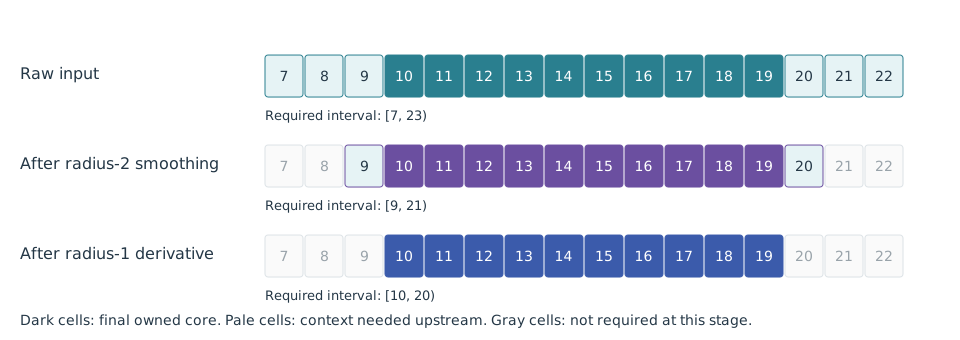
For compatible coordinate spaces, Reach::add combines sequential support side by side. A radius-two smoother followed by a radius-one derivative needs radius three on the original input. Reach::max combines independent branch requirements, but a combine kernel’s own neighborhood must also be included. Different coordinate spaces cannot simply be added; a new phase or explicit mapping is needed.
Iteration needs a further distinction. Several local updates fused inside one block can make the dependency grow with the number of updates. The older DeconvolveOp accounts for its fixed iteration count with reach proportional to twice the PSF radius times the count. A state-exchanging solver can instead synchronize after each pass and use just that pass’s support. The finite-PSF RL/SHB solver takes that route with disk-backed state available.
For a true fixed point, there is no known finite number of passes in general. IterativeOp expresses substage-by-substage image dependencies and a stopping rule; a local halo does not eliminate the need for state synchronization or convergence detection. Its current generic executor also retains whole-volume state. See fixed points and iterative execution for the operations that need this and why their dependencies cannot be replaced by one arbitrary finite overlap.
Choosing a block size after the dependency is correct
For a cubic interior core with edge b and symmetric halo h, the read/core volume ratio is ((b+2h)/b)^3. For b=32,h=8, it is 3.375; for b=128,h=8, it is about 1.424. This counts geometric input volume, not unique disk bytes: neighboring reads can share cached chunks. For anisotropic support, use the product of the three axis-specific ratios.
First choose the algorithm, boundary convention and required support. Then compare block shapes, tile alignment, phase composition and concurrent task counts. A larger halo can be a safe but expensive grant; a smaller required reach is a different algorithm unless the dependency derivation justifies it. The planner prices these choices and the correctness checks ensure that the committed output still covers the intended image.